GISAXS

Raw data & link to the electronic notebook

INSIGHT also provides tools for exporting and analyzing GISAXS data.

The workflow starts from TIFF files corresponding to the detector images acquired during the experiment. To adapt the notebook to your own dataset, you will need the experimental parameters provided by your beamline scientist, such as the wavelength, PONI coordinates, sample-to-detector distance, and incidence angle. These parameters can also be found in the PDF electronic notebook generated during the experiment.

The first cell contains all the beamline and detector parameters. Update the values if necessary, then run the cell.

# Modify with the beam parameters

# Geometry convention:
# PONIx / PONIy : direct beam position in detector pixels
# delta         : detector in-plane rotation angle (deg)
# gamma         : detector out-of-plane angle (deg)
# incidence_angle: grazing-incidence angle (deg)

wavelength = 1.55 # Angstrom
sample_detector_distance = 4445 # mm
PONIx = 490.5 # pixel
PONIy = 954 # pixel
delta = 0. # deg
gamma = 0. # deg
incidence_angle = 0.23 # deg
pixel_size = 0.172 # mm
detector_dimensions = (1043,981) # pixels

# Modify with the path to your image
path = "raw_data/SIRIUS_2021_10_15_2469_pilatus_sum.tiff"

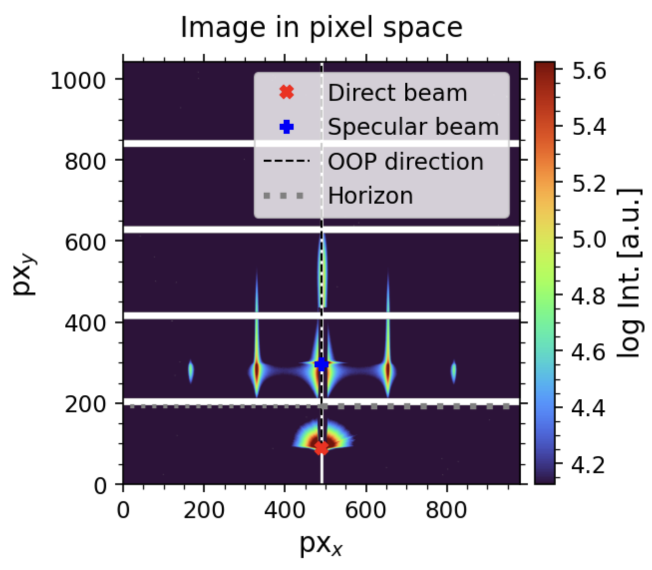
The next cell calculates the experimental geometry and displays the detector image in pixel coordinates. In most cases, it can be run without modification.

# Run this cell as is

def set_params_GISAXS(path):
    beam_params = {
     'db_x': detector_dimensions[1]-(PONIx-sample_detector_distance/pixel_size*np.tan(delta*np.pi/180.)),
     'db_y': detector_dimensions[0]-(PONIy+sample_detector_distance/pixel_size*np.tan(gamma*np.pi/180.)),
     'sdd': sample_detector_distance,
     'inca': incidence_angle,
     'px_size': pixel_size,
...

The resulting image is displayed in detector pixel coordinates.

GISAXS in reciprocal space and integration

The next step is to convert the detector image into reciprocal space coordinates (qy-qz). Unlike GIWAXS, GISAXS analysis generally does not require calculation of qx or correction for the curvature of the Ewald sphere.

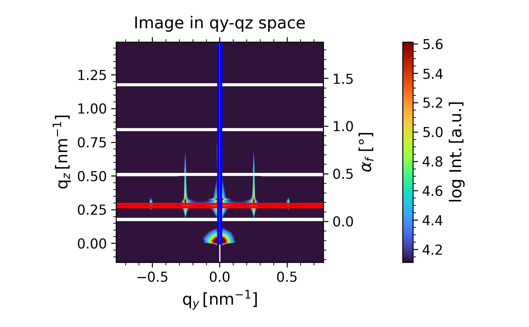
In the following cell, you can define the regions used for in-plane and out-of-plane integrations.

# Modify the parameters, and run the cell

# Define the qy integration range used to obtain the out-of-plane (qz) profile
# -> Blue rectangle
qy_center = 0. # qy-center of the integration range (in nm^-1)
qy_width = 0.002  # Width of integration range (in nm^-1)

# Define the qz integration range used to obtain the in-plane (qy) profile
# -> Red rectangle
qz_center = 0.028 # qz-center of the integration range (in nm^-1)
qz_height = 0.002  # Height of integration range (in nm^-1)

bin_number = 800 # Bin number for the GISAXS map

The transformed GISAXS map is displayed in reciprocal space together with the integration regions.

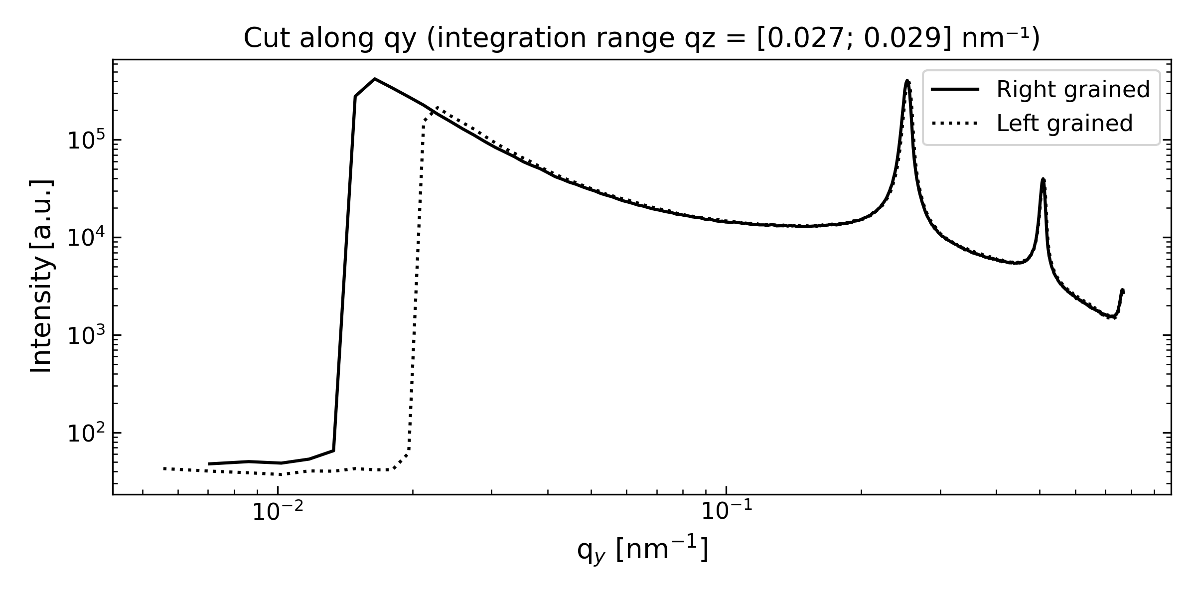
The in-plane (qy) profile is obtained by integrating over the selected qz range (red rectangle).

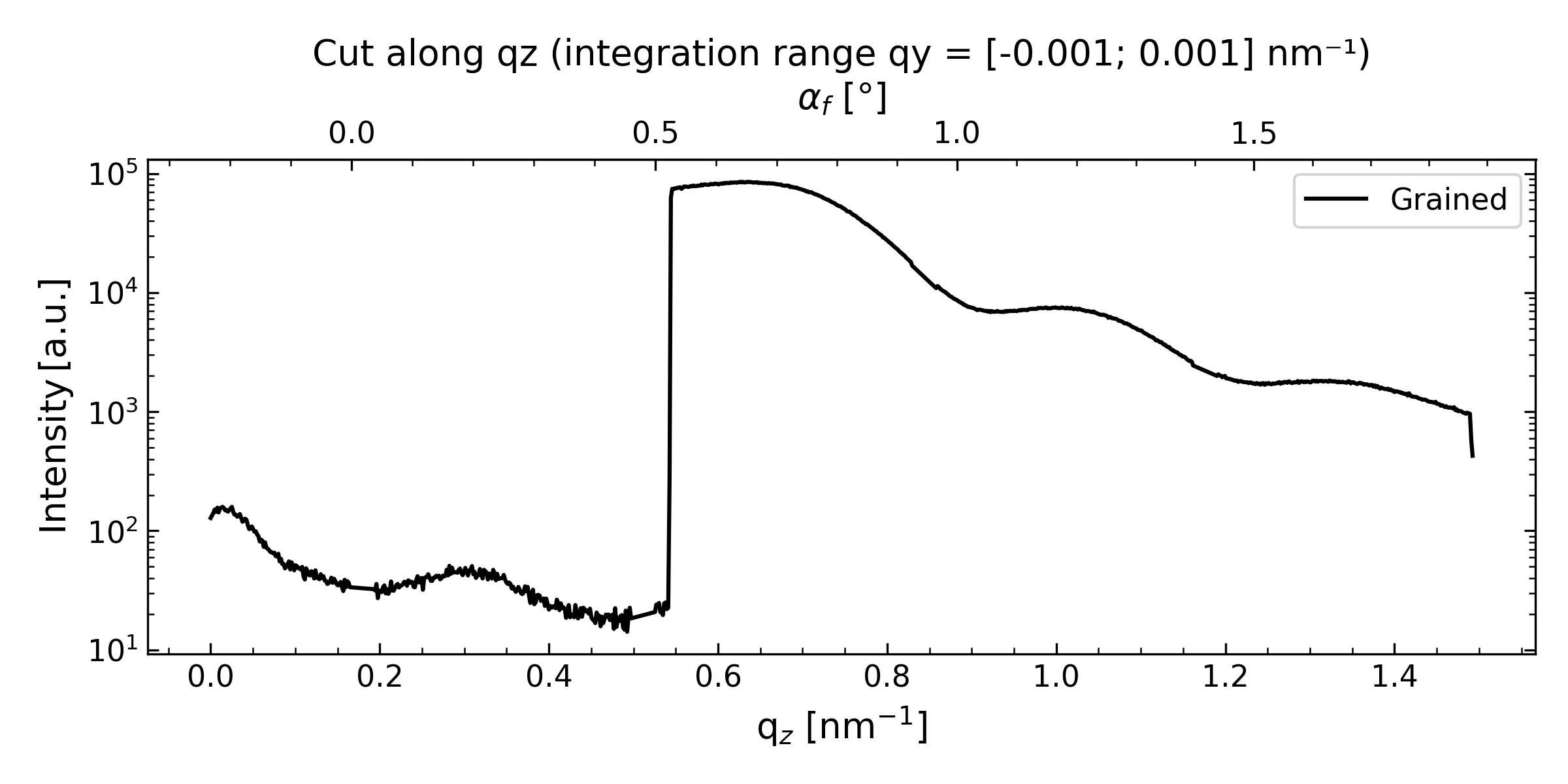
The out-of-plane (qz) profile is obtained by integrating over the selected qy range (blue rectangle).