Fit the data

To fit the data with the model, we first define which parameters can vary and set their bounds. For example, here we allow the roughness of the water layer to vary between 0.5 and 7 Ångströms:

water_bulk.rough.setp(bounds=(0.5, 7), vary=True)

To vary the thickness of a layer, we would use thick instead of rough, as shown below:

slab.thick.setp(bounds=(2, 5), vary=True)

The background value can also be fitted, using, for example:

water_bulk.rough.setp(bounds=(0., 1e-6), vary=True)

Next, we set up the fit with a \(\chi^2\) computed over the log of the reflectivity, and use a differential evolution algorithm. Other methods are described here.

objective = Objective(model, data_exp, transform=Transform("logY"))
fitter = CurveFitter(objective)
fitter.fit("differential_evolution")

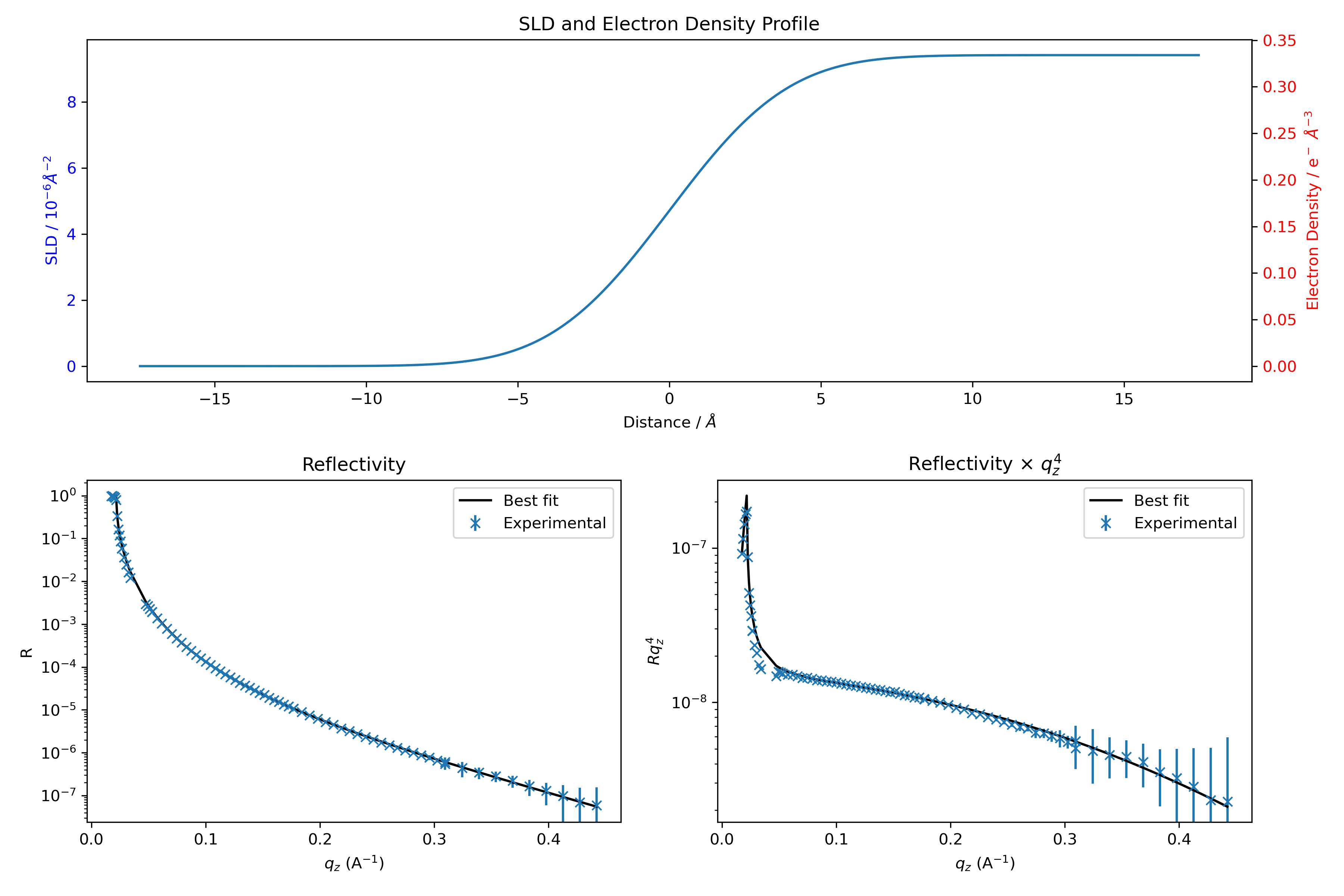
A list of fitting details is printed, along with a plot showing the best-fit result. Additionally, a list of varying parameters with their final values is shown. Keep in mind that if you run this cell again, the initial guess will now be based on the last fit result.

If you are satisfied with the result, run the next cell to save the curve and SLD in a CSV file.

# Prepare the data to be saved
data_to_save = np.column_stack((qz_exp, R_model, R_exp, R_err_exp))

# Save the data to the text file
np.savetxt(f'{folder_path}/fit-result.dat', data_to_save, header="qz(A^-1) R_model R_exp R_err_exp", fmt="%.6e")

# Extract SLD profile data
z, sld = stack.sld_profile()

# Calculate electron density
ed = sld_to_ed(sld)

# Combine into a single array with three columns: z, SLD, ED
sld_ed_to_save = np.column_stack((z, sld*1e-6, ed))

# Save to a text file
np.savetxt(f'{folder_path}/sld-profile.dat', sld_ed_to_save,
           header="Distance(A) SLD(A^-2) EDP(e-/A^3)",
           fmt="%.6e")