More complex example: a lipid monolayer#
We now proceed with a more complex system than a simple liquid–gas interface. We will build the model step-by-step and estimate initial guesses for the various parameters.
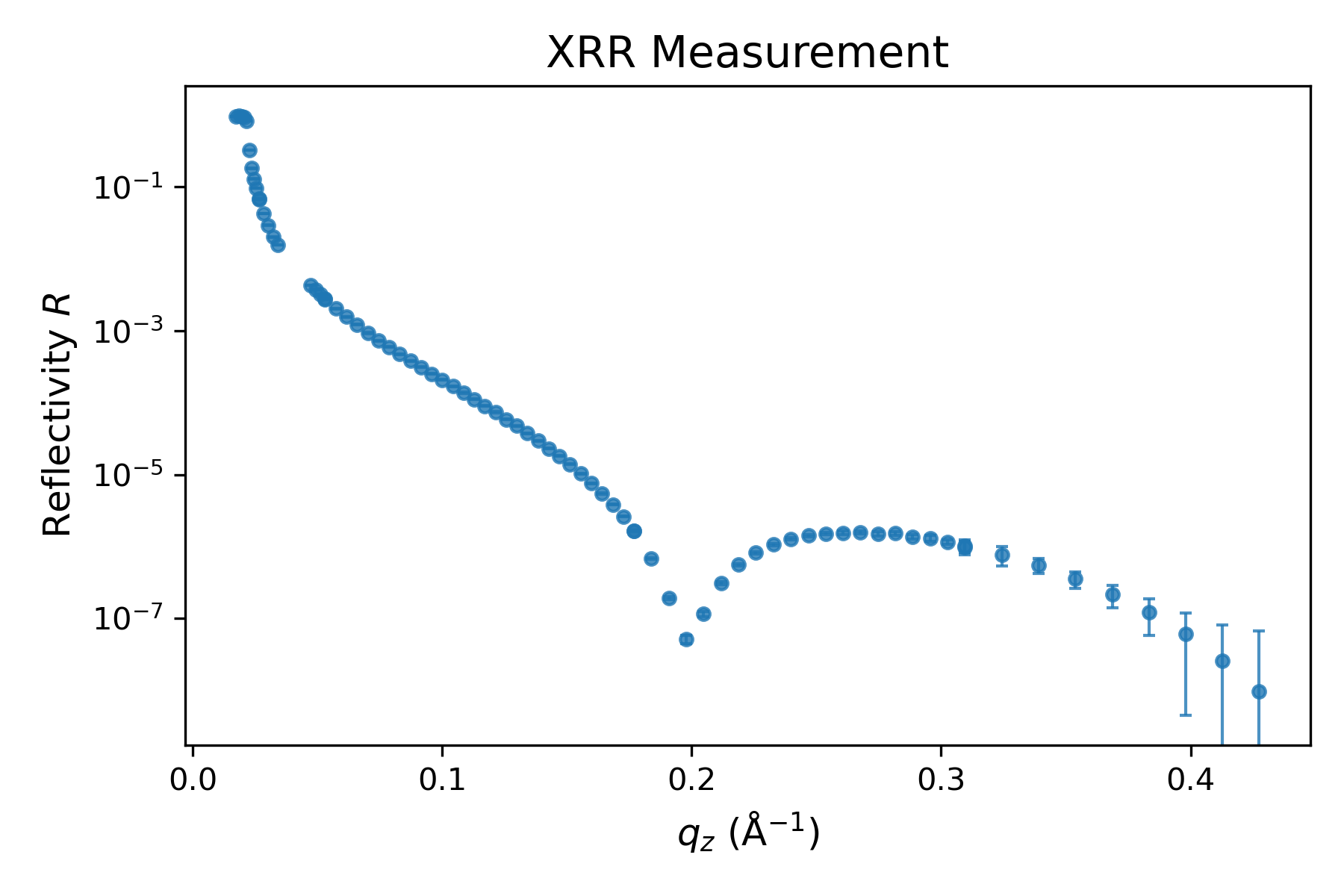
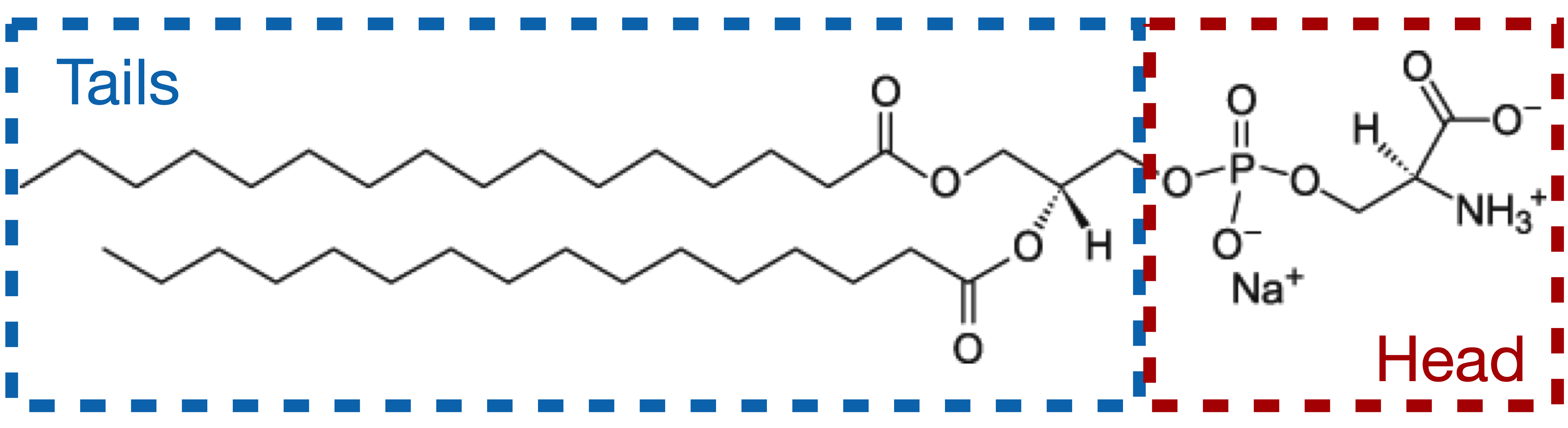
The data correspond to a monolayer of the phospholipid DPPS (1,2-Dipalmitoyl-sn-glycero-3-phosphoserine, 16:0/16:0 PS), at the helium-water interface, at an area-per-molecule of 0.38 nm\(^2\) (surface pressure of 40 mN/m).
Import data#
We import and filter the data in the same way as before.
# Path to the XRR file
path_XRR = 'raw_data/SIRIUS_2024_09_20_4556-4640_XRR.dat'
...
Create the model#
The signal measured in XRR is dictated by electron density contrast between the different layers. As such, it would be incorrect to model the lipid as a single block, as the aliphatic chains and the PS head exhibit a strong density contrast. Therefore, we will model our system with the following layers, from top to bottom:
a semi-infinite medium of Helium (considered as vacuum),
a layer for the aliphatic tails,
a layer for the PS heads,
a semi-infinite sub-phase of water.
Tail layer#
We estimate initial values for each parameter as follows:
Thickness \(d\)#
A good starting point for the thickness of the tail layer is the theoretical length of an elongated aliphatic chain with \(n\) carbons in all-trans conformation, given by [8, 9]:
or, considering gauche defects:
In this case, we have 16 C per chain, yielding \(L_{\rm max} = 22\) \(\rm A\). We’ll use this as our initial thickness guess.
Electron density \(\rho_{el}\)#
In our model, the chains are composed of 35 C, 67 H, and 4 O atoms. We can use the area per molecule from the Langmuir trough \({\cal A} = 38\) \({\rm A}^2\) and the estimated layer thickness \(d = 22\) \(\rm A\) to calculate the density. Since we consider two chains per molecule, the electron density is:
This is likely an overestimate (the chain density should be slightly lower than that of water), but serves as a reasonable starting point.
Roughness \(\rm \sigma\)#
A typical initial guess is \(\sigma = 3\) Å, as observed for the water interface.
Head layer#
Thickness \(d\)#
Looking at the chemical drawing of our molecule, we estimate a minimum thickness of approximately 5 \(\rm A\).
Electron density \(\rho_{el}\)#
In our model, the heads are composed of 3 C, 6 H, 6 O, 1 P, 1 Na, and 1 N atoms. Using the same approach as before to calculate the electron density:
Roughness \(\rm \sigma\)#
We again use an initial value of \(\sigma = 3\) \(\rm A\).
Sub-phase#
We set the initial roughness of the water subphase to \(\sigma = 3\) \(\rm A\).
Code#
All-in-all the code for constructing the model is:
## DEFINE SLDs

# Electron density in e-/A^3
rho_water = 0.334
rho_helium = 0.
rho_tail = (35*6+67+4*8)/(38*22)
rho_head = (3*6+6+6*8+15+11+7)/(38*5)

# Conversion to SLD = r_el*rho_el
# SLD in refnx should be in 1e-6 A^-2
r_el =  2.81794e-5 # in A
SLD_water = rho_water*r_el*1e6
SLD_helium = rho_helium*r_el*1e6
SLD_tail = rho_tail*r_el*1e6
SLD_head = rho_head*r_el*1e6

# Define a medium by its SLD
water = SLD(SLD_water, name = 'water')
helium = SLD(SLD_helium, name = 'helium')
tail = SLD(SLD_tail, name = 'tail')
head = SLD(SLD_head, name = 'head')

## DEFINE EACH SLAB

# All lengths in A
# First number is the thickness
# Second number is the roughness (with respect to the top layer)

# Semi-infinite bulk : thickness := 0
water_bulk = water(0, 3)

tail_slab = tail(22, 3)
head_slab = head(5, 3)

# Semi-infinite bulk : thickness := 0
helium_atm = helium(0, 0)


## CONSTRUCT THE STACK

# From top to bottom
stack = helium_atm | tail_slab | head_slab | water_bulk

## SIMULATE XRR

model = ReflectModel(stack, bkg=0, dq=0.1)
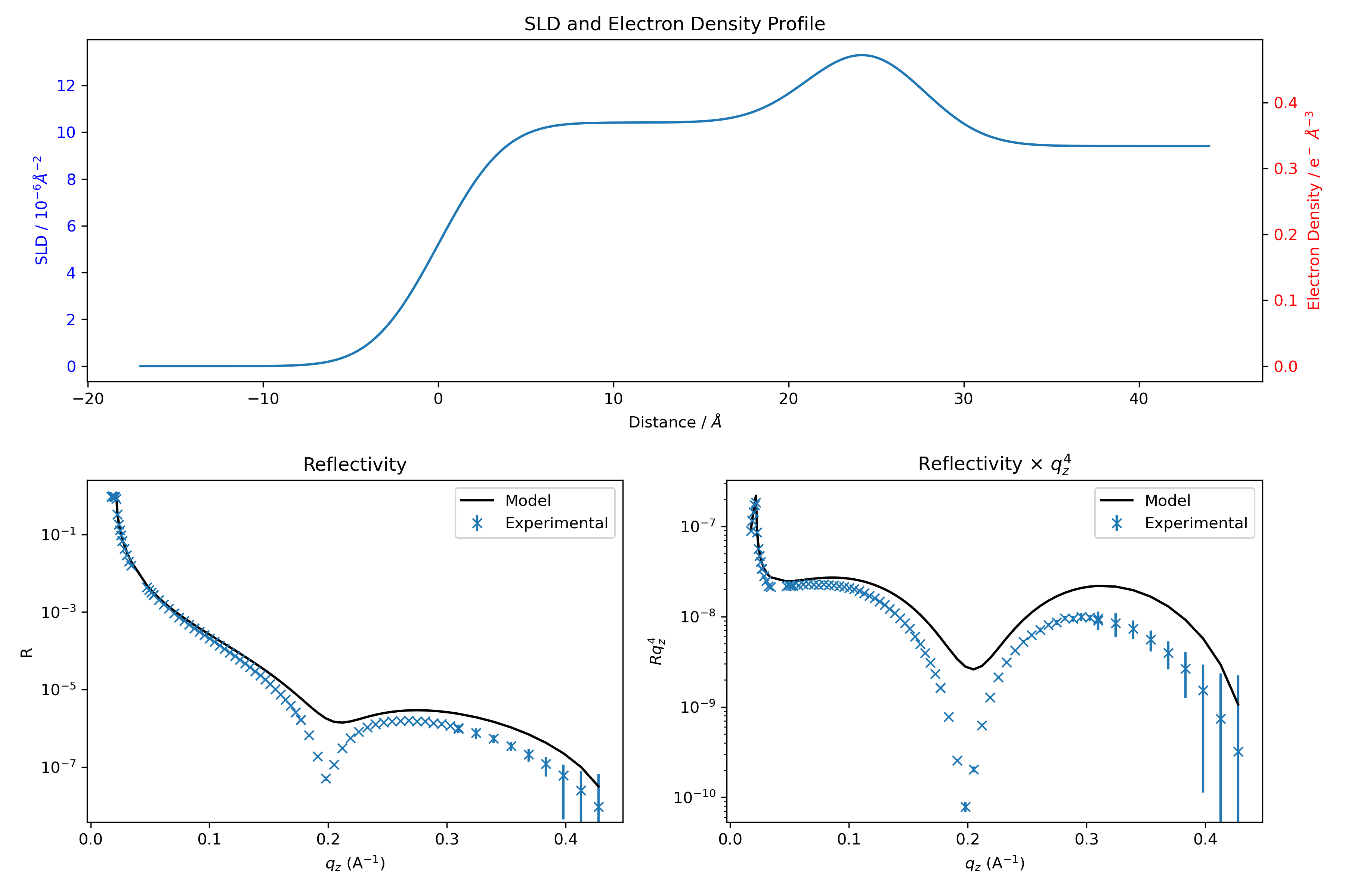
This leads to the following initial guess:
Define fitting parameters#
We specify the parameters to vary and their bounds:
\(\sigma_{\rm tail}\) and \(\sigma_{\rm head}\) between \(2\) and \(6\) \(\rm A\),
\(\sigma_{\rm water}\) between \(2\) and \(4\) \(\rm A\),
\(d_{\rm tail}\) between \(16\) and \(25\) \(\rm A\),
\(d_{\rm head}\) between \(5\) and \(11\) \(\rm A\).
The densities are allowed to vary within \(\pm\) 25 \(\%\) of their original value.
## DEFINE FIT PARAMETERS

water_bulk.rough.setp(bounds=(2, 4), vary=True)
tail_slab.rough.setp(bounds=(2, 6), vary=True)
head_slab.rough.setp(bounds=(2, 6), vary=True)

tail_slab.thick.setp(bounds=(16, 25), vary=True)
head_slab.thick.setp(bounds=(5, 11), vary=True)

tail_slab.sld.real.setp(bounds=(SLD_tail*0.75, SLD_tail*1.25), vary=True)
head_slab.sld.real.setp(bounds=(SLD_head*0.75, SLD_head*1.25), vary=True)


## FIT THE DATA

objective = Objective(model, data_exp, transform=Transform("logY"))
fitter = CurveFitter(objective)
fitter.fit("differential_evolution")
Fit result#
The fitting and plotting have been separated into two cells. This allows you to interrupt the fitting (e.g. if it takes too long) using the stop button in Jupyter. Errors will appear in the output, but the plot will still reflect the current state of the fit.
If the fitting completes successfully, you should see excellent agreement between model and experiment:
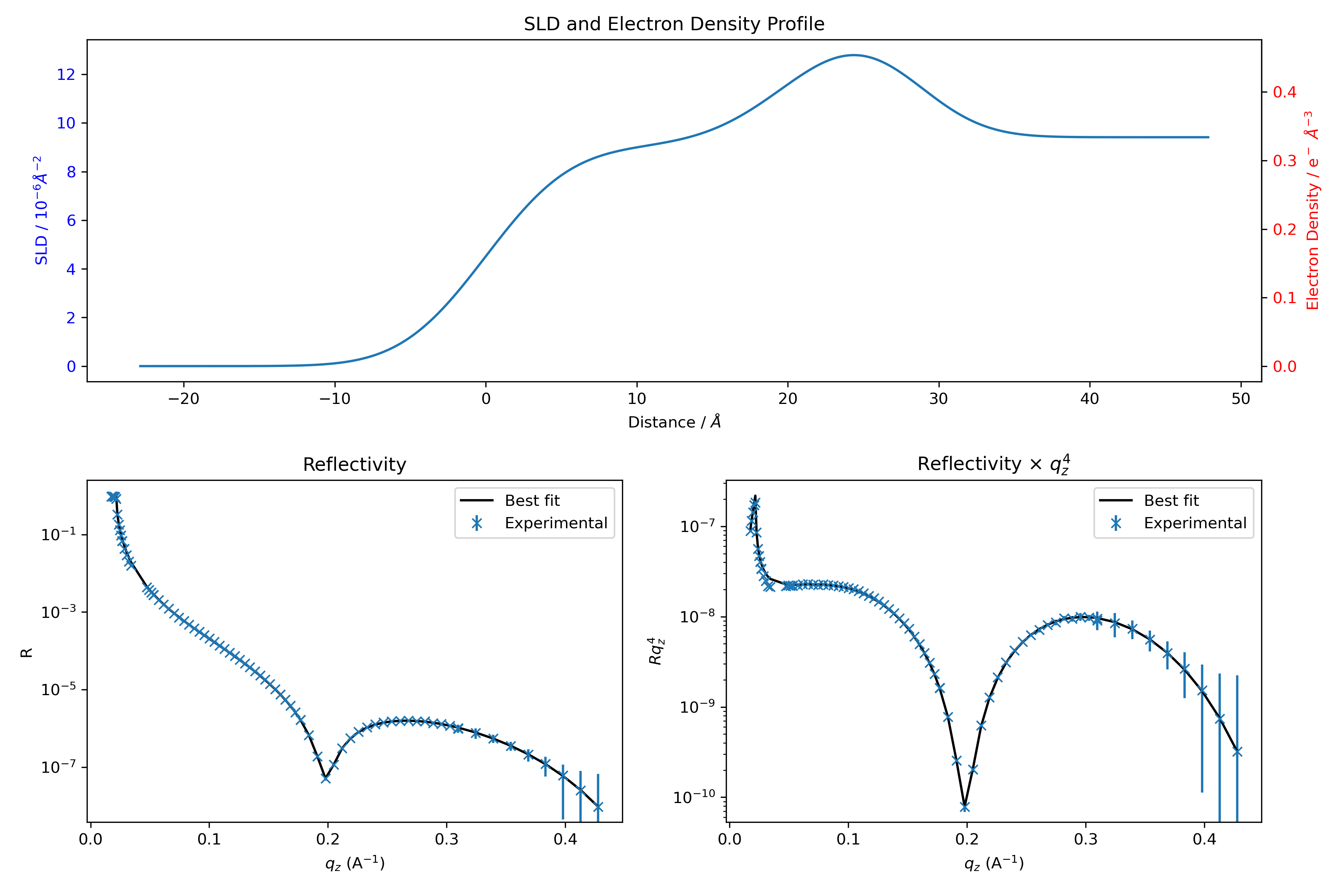
Be careful, this does not necessarily mean that you have solved the structure of your sample. You have found one set of parameters that fit the data, but there is no guarantee that another set of parameters would not fit the curve equally well (an inherent limitation of XRR).
Error bars#
Caution should be exercised when interpreting the error bars resulting from this fitting procedure. These uncertainties may not fully capture the true variability or correlations in the model parameters.
If more accurate or statistically robust error estimation is required, alternative methods—such as Bayesian inference using MCMC or nested sampling—should be considered. These approaches are beyond the scope of this tutorial, but are documented here.