Create a model#
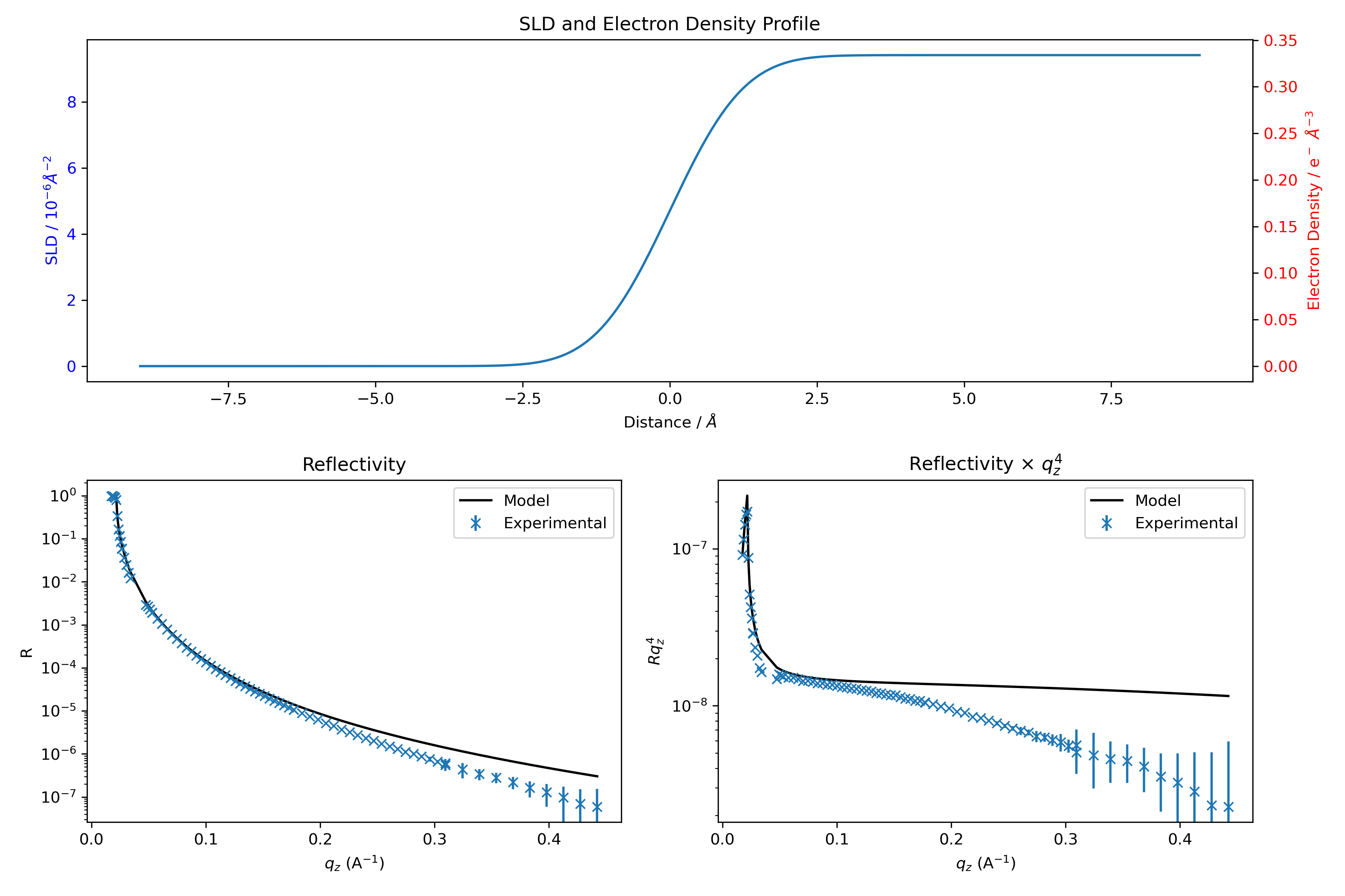
The next cell creates a very simple model for this first part of the tutorial. It consists of a semi-infinite bulk of helium atmosphere on top of a semi-infinite bulk of water. There is only one tunable parameter: the roughness of the interface. Here, we build an initial guess for the model, which we will later compare with and fit to the experimental data.
Define SLDs#
First, we need to define the SLDs (Scattering Length Densities) of the materials. refnx expects SLDs to be in units of \(10^{-6} \, A^{-2}\). However, it is often more convenient and intuitive to work with electron densities in \(e^{-}/A^3\). We therefore define the electron densities of the two media at the beginning of the cell, and later convert them to units suitable for refnx.
# Electron density in e-/A^3
rho_water = 0.334
rho_helium = 0.

# Conversion to SLD = r_el*rho_el
# SLD in refnx should be in 1e-6 A^-2
r_el =  2.81794e-5 # in A
SLD_water = rho_water*r_el*1e6
SLD_helium = rho_helium*r_el*1e6

# Define a medium by its SLD
water = SLD(SLD_water, name = 'water')
helium = SLD(SLD_helium, name = 'helium')
Define each slab#
Next, we define each slab that will be used in the final stack. In this case, we need two slabs: one for each semi-infinite medium. The first number represents the slab thickness (set to 0 for a semi-infinite medium) in Ångströms, and the second is the roughness with respect to the layer above it.
# All lengths in A
# First number is the thickness
# Second number is the roughness (with respect to the top layer)

# Semi-infinite bulk : thickness := 0
water_bulk = water(0,1)

# Semi-infinite bulk : thickness := 0
helium_atm = helium(0,0)
Construct the stack#
We construct the stack from top to bottom, using `| to separate each slab.
# From top to bottom
stack = helium_atm | water_bulk
Simulate XRR of initial guess#
Finally, the XRR corresponding to this initial guess is calculated and plotted against the experimental data.
model = ReflectModel(stack, bkg=0, dq=0.1)
We assume that the background correction is perfect and the background can be set to zero. We use a constant intrumental resolution of \(dQ/Q=0.1\%\) that is usually sufficient to describe experimental data. See here if a more complex resolution function is needed.