Sample parameters#
Now we will learn through the same simple example what each parameter means, how you can tune them, and how the different displays work.
Sample tab#
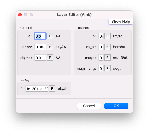
The sample tab is where you create your model. In our example, you will notice that there are only two semi-infinite layers: the substrate (actually a sub-phase) Sub and, above it, the atmosphere Amb. We will see how to add an extra layer in a future section. For now, let’s focus on the meaning and options of each parameter.
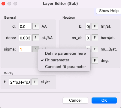
To open the sample editor, double-click on one of the layers. In this editor, you can change parameter values and define whether a parameter is a constant or a fit parameter by clicking on the F symbol.
Parameters of each layer#
Thickness#
The layer thickness is represented by d, in angströms. Leave the value as \(0\) for the semi-infinite top and bottom media.
Density#
The density (parameter dens) in GenX is arguably the most challenging parameter to understand. The unit is the density of formula units, expressed in units per \(\rm{A}^3\). This choice of units is well-suited for systems relevant to hard-condensed matter but less intuitive for soft matter. Here are two examples to illustrate this unit:
A crystal of \(\rm SrTiO_3\) with a cubic structure of parameter \(a = 3.9045 \, \rm{A}\). You have one formula unit (\(\rm SrTiO_3\)) per \(a^3\), so the density in the units required by GenX is \(1/3.9045^3 = 0.0168\).
A Body-Centered Cubic (BCC) structure of \(\rm Fe\). This structure contains two formula units (\(\rm Fe\)) per \(a^3\), so the density is \(2/a^3\).
In soft matter systems, however, a crystal is not necessarily present. A useful relation for these systems is:
where \(\rho\) is the specific mass in \(\rm{kg/m^3}\), and \(\rm{u_{scatt}} = \sum_i u_i x_i\) is the linear combination of the individual atomic masses of each element.
Example: \(\rm H_2O\)#
For example, for \(\rm H_2O\):
\(\rho = 1 \, \rm{g/cm^3} = 1000 \, \rm{kg/m^3}\),
\(\rm{u_{scatt}} = 2 \times 1.008 + 1 \times 15.999 = 18.015\),
and the density in the appropriate units is:
Example: \(\rm SrTiO_3\)#
We can recover the result obtained with \(\rm SrTiO_3\) using this new approach:
\(\rho = 5.12 \, \rm{g/cm^3}\),
\(\rm{u_{scatt}} = 1 \times 87.62 + 1 \times 47.87 + 3 \times 16 = 183.49\),
and the density in the appropriate units is:
Link with the electron density: example of a lipid head#
We will deal more precisely with the case of a lipid at the gas-water interface in the section Build a more complex model. But we will use the opportunity of this tutorial to make the link between GenX density and a more natural unit for density in XRR studies of soft matter systems, the electron density, \(\rho_{el}\) (number of electrons per unit volume). A useful reference is the electron density of water: \(\rho_{el} = 0.33 \, \rm{e}^{-}/\rm{A}^{3}\). Later in this tutorial, you will see that one of the outputs of GenX is the electron density profile, which provides \(\rho_{el}\) as a function of \(z\), the depth in your sample.
If you know the electron density in \(\rm{e}^{-}/\rm{A}^{3}\) and the number of electrons \({n_{el}}\) in the formula unit, the parameter dens can be calculated using:
For example, consider the head group of the phospholipid DSPC with the formula \(\rm{C_{10}H_{18}O_{8}NP}\). If we aim for an electron density of \(0.4 \, \rm{e}^{-}/\rm{A}^{3}\), we calculate:
Roughness#
The root mean square roughness of the top interface of a layer is parameterized by sigma. You can set the parameter sigma of the sub-phase as a fit parameter, which we will optimize later.
Formula#
The simplest way to use the f parameter (the x-ray scattering length per formula unit, in electrons) is to input the chemical formula of your layer as a linear combination of \(\rm fp\). For example, fp.Si + 2*fp.O for \(\rm SiO_2\) or 2*fp.H + fp.O for \(\rm H_2O\).

Neutrons#
Leave all the other parameters, which are relevant only for neutrons, set to \(0\).
If you’ve missed any steps, you can download the updated file here.