Calibration with a reference sample (optional)#
This section explains how to perform a calibration using Silver Behenate [17] to fine-tune the parameters of your experimental setup. This step is optional if the beamline scientist has already provided the beamline parameters for your experiment. However, it is always beneficial to verify that the sample-to-detector distance is accurate.
Open the calibration wizard by clicking on Tools > Calibration Wizard.
Load Image#
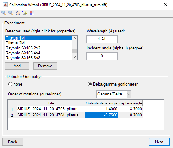
Select the image acquired during the calibration. If you have images taken at different detector angles, select all of them. For this example, we use two images:
4703: Taken at an out-of-plane detector angle \({\rm gamma} = -1.4\) degrees.
4704: Taken at \({\rm gamma} = -0.75\) degrees.
Geometry#
Verify that the parameters are correct. These should be extracted from your current experimental setup defined in the previous sections. The incident angle should be 0 for Silver Behenate measured in transmission. Assign the appropriate angles to each file.
Click on Next and confirm the warning pop-up by selecting Yes.
Start Parameters#
Review and adjust the parameters starting from the values provided in the notebook. Typically, the center positions are accurate, and you may need to optimize only the Sample detector distance. If your analysis requires greater accuracy, you can optimize additional parameters, but this is outside the scope of this tutorial.
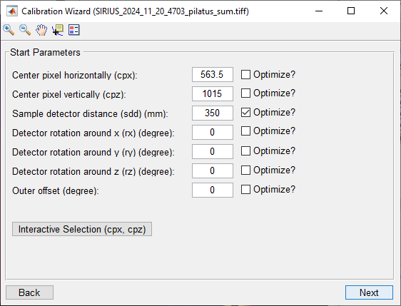
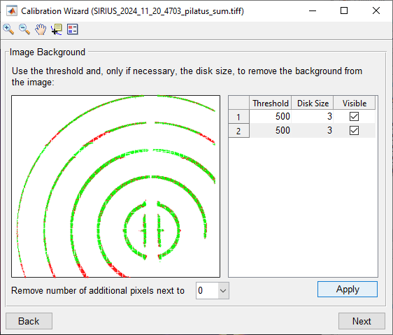
Image Background#
Adjust the background signal by modifying the available parameters. In most cases, the default starting point is sufficient. Use this step to count the number of visible rings (e.g., 5 in this example).
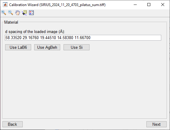
Material#
Select the calibration standard Use AgBeh to load the d-spacings for Silver Behenate. Retain only as many d-spacing values as there are visible rings, starting from the largest spacing. For this example, keep the first 5 values.
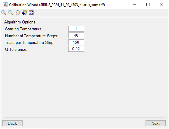
Algorithm Options#
Retain the default values except for Q Tolerance. Start with a value of \(0.02\). Adjust the tolerance as needed by switching back and forth between this window and the next one. The dotted lines should align closely with the rings without overlapping. A value of \(0.02\) is generally a good starting point.
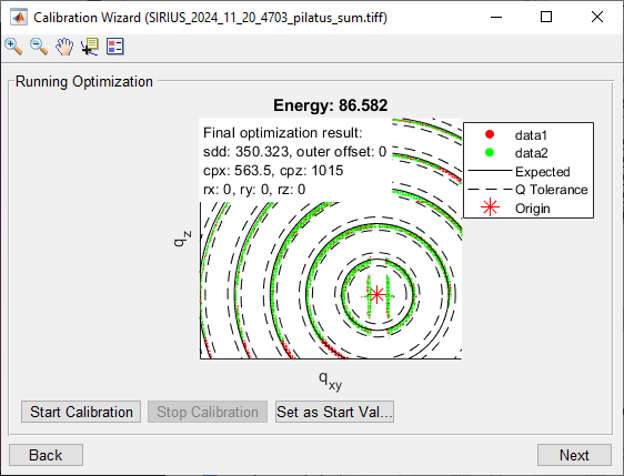
Running Optimization#
Click Start Calibration and wait for the optimization to finish. The optimized parameters will appear in the figure label. Record these parameters for later use.
Results#
You can save the results to your current beamtime setup. This will allow you to use them directly as an Experimental Setup in the Load File window.