In-plane and out-of-plane integration

In-plane and out-of-plane integration#

Warning: out-of-plane integration is often not rigorous#

With a single angle of incidence, it is impossible to fully cover the range of \(q_z\) at \(q_{xy}=0\) due to the limitations of measuring the Ewald sphere with a planar 2D detector [18].

To rigorously obtain the out-of-plane region of reciprocal space at \(q_{xy}=0\), other techniques should be used, such as diffraction in specular conditions.

An approximation often made is to ignore the corrections required by the Ewald sphere, and integrate on \(q_x\) vs. \(q_z\) maps. In this case, note that comparisons between in-plane and out-of-plane integrations are mostly qualitative, particularly at high \(q_z\) values.

We will see different approaches here to obtain in-plane and out-of-plane integrations.

Integration directly in q-space#

In-plane#

Performing in-plane integration directly in q-space is possible, since there is only little corrections related to the Ewald sphere.

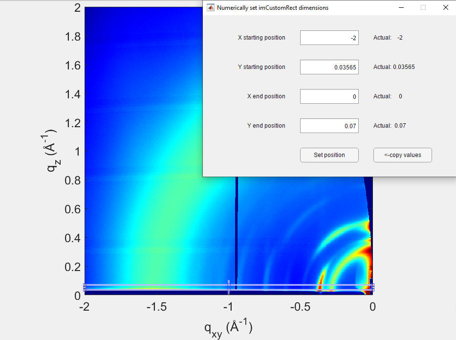
Initiate Integration: Click on the ILS (Integrated Line Scan) icon.
Draw the Integration Area: Draw a rectangle to define the integration region. Typically, this rectangle is positioned just above the Yoneda-Vineyard peak, near the critical angle of total external reflection.
- To adjust precisely, right-click the rectangle and select Set position.
- Keep the rectangle’s height consistent across samples for comparative purposes.
- Ideally, report the integration domain in publications.

Update Data: In the Integrated Line Scan window, click on Update Data to process the selected rectangle.

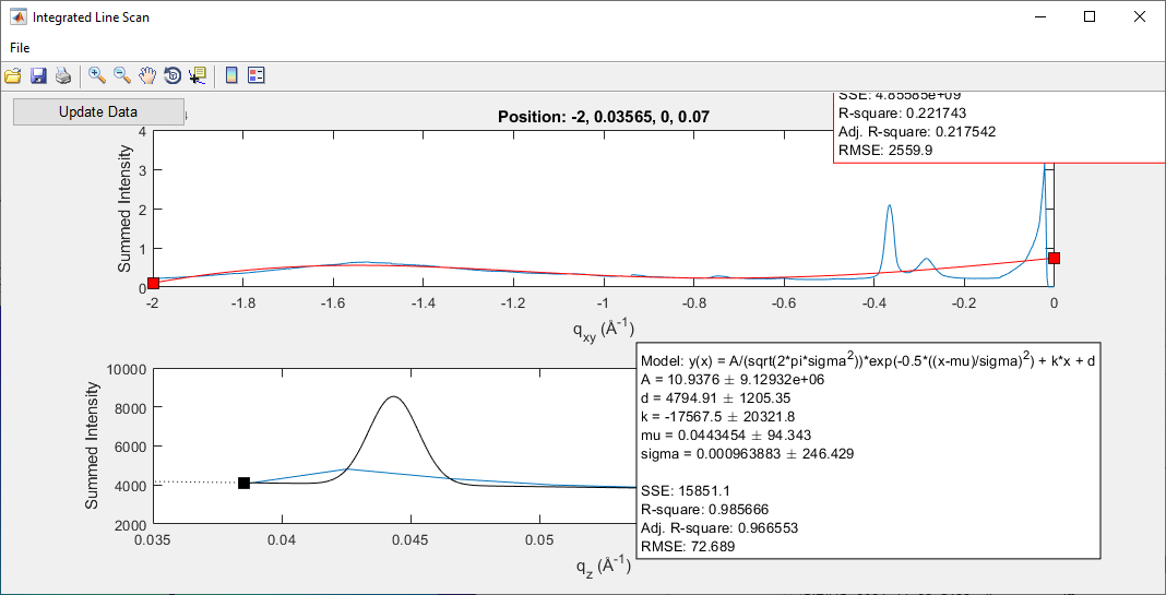
Export Data: If needed, fit the peak positions using GIDVis or export the data for external analysis.
- Go to File > Export Line Data....
- Select only Sum vertically, then click on Export and Close.

The exported text file contains intensity as a function of \(q_{xy}\) in a two-column format. For this tutorial, the file was saved as 5151-5152-direct-integration-qxy.txt.

Out-of-plane#

Due to the missing wedge, the out-of-plane integration directly in q-space is limited to small \(q_z\) only. In our example, that would be up to \(\sim 6\) \(\rm{nm}^{-1}\).

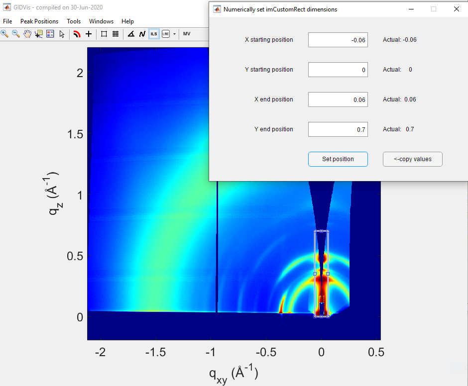
Initiate Integration: Click on the ILS (Integrated Line Scan) icon.
Draw the Integration Area: Draw a rectangle to define the integration region. Typically, this rectangle is centered on the beamstop.
- To adjust precisely, right-click the rectangle and select Set position.
- Keep the rectangle’s height consistent across samples for comparative purposes.
- Ideally, report the integration domain in publications.

Update Data: In the Integrated Line Scan window, click on Update Data to process the selected rectangle.

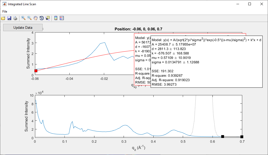
Export Data: If needed, fit the peak positions using GIDVis or export the data for external analysis.
- Go to File > Export Line Data....
- Select only Sum horizontally, then click on Export and Close.

The exported text file contains intensity as a function of \(q_{z}\) in a two-column format. For this tutorial, the file was saved as 5151-5152-direct-integration-qz.txt.