Azimuthal scan

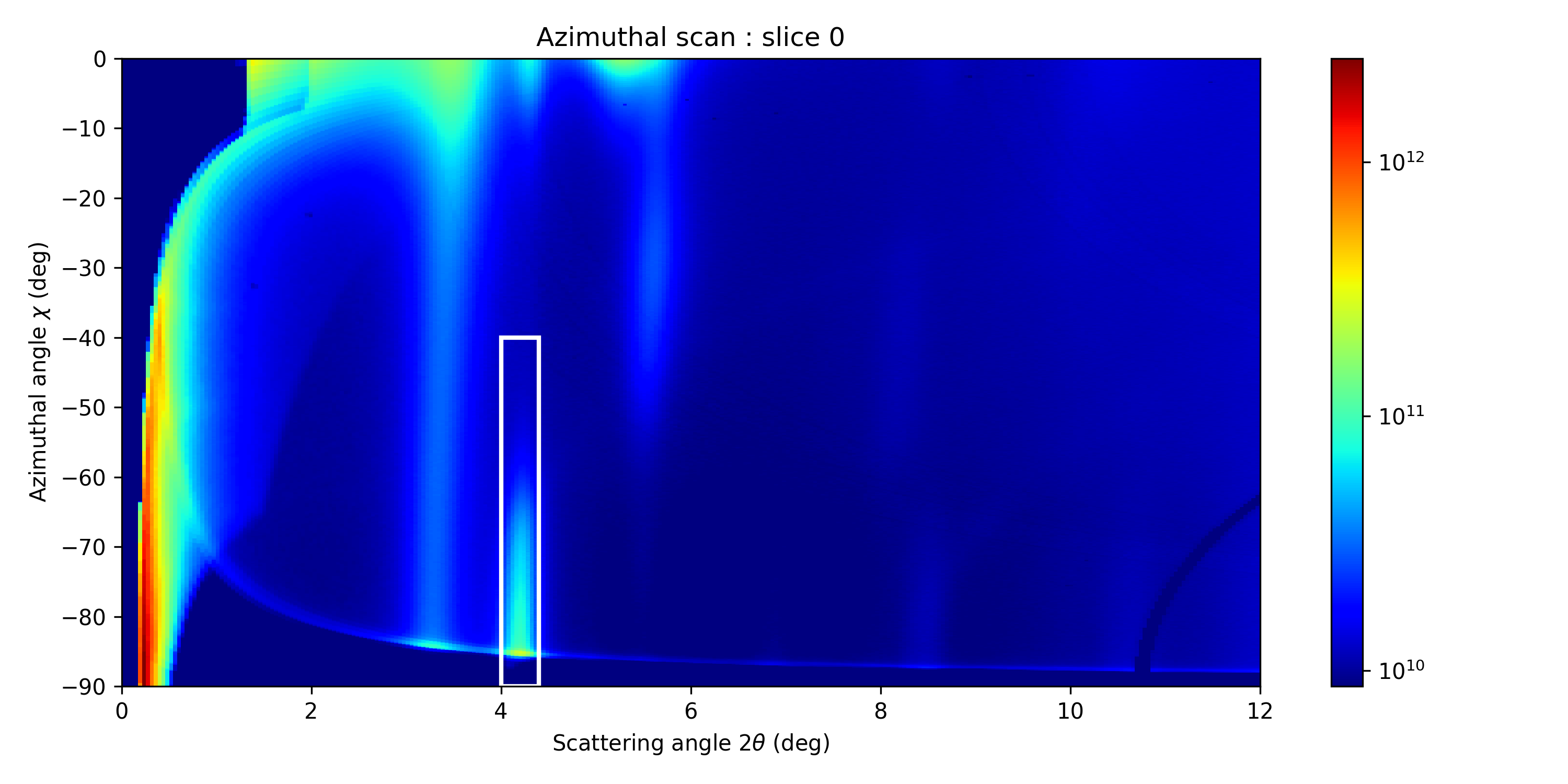
Azimuthal vs 2\(\theta\) map

In this step, we will extract the azimuthal scan, which is useful for analyzing texturing effects. First, we generate the azimuthal vs. 2\(\theta\) map, where we will define the integration region for the scan.

You can adjust the maximum 2\(\theta\) value to be displayed in the image, then run the cell.

# Modify only the maximum 2_theta you want to reach in the image, and run the cell
max_tth = 12 #in-plane, in deg

...

Running the cell will generate the map.

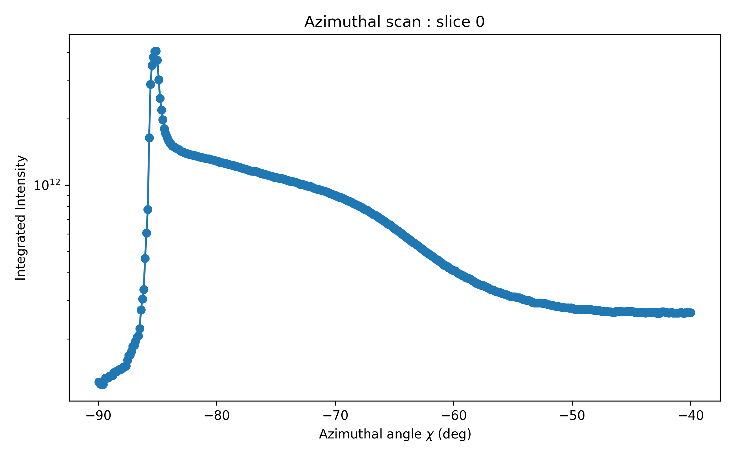
Azimuthal scan

Now, we need to define the integration region on the 2D map to obtain the intensity vs. azimuthal angle (\(\chi\)) plot.

You can adjust the integration boundaries (represented by the borders of the white rectangle) and then run the cell.

# Modify only the limits for the integration, and run the cell.

# Define the left and right boundaries for selection (modify these values)
left_tth = 4.    # Set your desired left boundary (in degrees)
right_tth = 4.4  # Set your desired right boundary (in degrees)
# Define the top and bottom chi boundaries
bottom_chi = -90   # Bottom boundary (in degrees)
top_chi = -40      # Top boundary (in degrees)

...